DOI:
10.13140/RG.2.2.10484.41608
The Semiconductor Supply chain is diversifying from South East Asia to South Asia. Covid 19 and Trade war between USA -China are the primary factors driving this shift. Developing countries such as Thailand, Indonesia, Cambodia, Malaysia etc are pushing hard to attract companies with varieties of Policies.
India launched its semiconductor mission in 2022 . India’s first private sector fabrication company TATA Electronic is a joint venture between TATA and PSMC , it will be operational by 2026. As of Jan 2026 there are a total of 9 OSAT plants in India and 1 fabrication plant. Present study analyzes the Geographical parameter that affects the economies of different plants in India. They Study is based on Indian meteroloical data.
Following climatic factors affect the Semiconductor Plant;
- Temperature-
- Humidity-
- Water Availability-
Data Source
Present study is based on Data available on IMD Portal. (1991-2020)
Table 1: climatological data (03 utc and 12 utc)
| Stations | Ahmedabad 03 | Ahmedabad 12 | Tirupati 03 | Tirupati 12 | Bhubaneswar 03 | Bhubaneswar 12 | Guwahati 03 | Guwahati 12 |
| Mean station pressure (hPa) | 1003.8 | 1000.3 | 998.3 | 994.4 | 1004.2 | 1000.9 | 1004.4 | 1000.4 |
| Dry bulb temperature (°C) | 24.4 | 32.7 | 27.1 | 31.9 | 26.5 | 28.5 | 24 | 26.5 |
| Wet bulb temperature (°C) | 20.3 | 22.6 | 23.2 | 24.1 | 23.9 | 24.3 | 21.8 | 22.8 |
| Relative humidity (%) | 67 | 41 | 71 | 52 | 79 | 70 | 81 | 72 |
| Vapour pressure (hPa) | 21.7 | 20.1 | 25.5 | 23.9 | 28.3 | 27.6 | 25.2 | 25.6 |
| Total clouds (okta) | 2.8 | 2.8 | 4.6 | 4.8 | 3.9 | 4.2 | 4.3 | 4.4 |
| Low clouds (okta) | 1.3 | 1.4 | 1.7 | 2.2 | 2.1 | 2.2 | 2.4 | 2.4 |
03 utc represents baseline morning conditions, while 12 utc evening captures peak thermal stress. Ahmedabad shows the largest temperature rise and strongest daytime drying, indicating intense sensible heat gain. Bhubaneswar and Guwahati show small temperature rise but persistently high vapour pressure, confirming dominance of latent (moisture) load.
The analysis uses mean daily maximum temperature (Tmax)to represent sustained thermal load and extreme maximum temperature (Text)to capture peak heat stress conditions. Diurnal temperature rise (ΔT)is defined as the difference between dry bulb temperature at 12 utc and 03 utc and reflects daytime sensible heat gain. Atmospheric moisture conditions are represented by vapour pressure at 12 utc (e) and relative humidity at 12 utc (RH), which together indicate latent cooling and dehumidification demand. Water availability is characterised by rainy days per year (RD) and precipitation reliability (PR), calculated as RD divided by 365, serving as a proxy for water security. mean wind speed (WS) represents background air movement, while fog days (FD) and thunder days (TD) are used to capture climate-related operational disruption risk.
Table 2: Annual temperature, rainfall, and wind characteristics
| Stations | Ahmedabad | Tirupati | Bhubaneswar | Guwahati |
| Mean daily maximum temperature (°C) | 34.4 | 34.8 | 33 | 30 |
| Mean daily minimum temperature (°C) | 21.2 | 23.9 | 22.4 | 19.7 |
| Highest maximum temperature (°C) | 44.7 | 43.9 | 43.6 | 37.8 |
| Lowest minimum temperature (°C) | 7.2 | 14.9 | 10.7 | 7.7 |
| Annual rainfall (mm) | 783.6 | 1113.5 | 1657.8 | 1695.3 |
| Rainy days (number) | 33.9 | 55.1 | 72.9 | 90 |
| Mean wind speed (kmph) | 7.2 | 6.5 | 5.6 | 1.9 |
Table 3: Extreme and event-based climate indicators
| Stations | Ahmedabad | Tirupati | Bhubaneswar | Guwahati |
| Days with precipitation ≥ 0.3 mm | 52.3 | 82.5 | 99.7 | 129.1 |
| Days with hail | 0 | 0.1 | 0.2 | 0.7 |
| Days with thunder | 23 | 23.6 | 21.3 | 70.7 |
| Days with fog | 1.9 | 4.8 | 8.2 | 28.5 |
| Days with dust storm | 0.9 | 0 | 0 | 0.6 |
| Days with squall | 1.8 | 0 | 0 | 1.4 |
Table 4: Derived diurnal and moisture metrics (from 03–12 utc)
| Stations | ΔT (°C) | Δ vapour pressure (hPa) |
| Ahmedabad | 8.3 | −1.6 |
| Tirupati | 4.8 | −1.6 |
| Bhubaneswar | 2 | −0.7 |
| Guwahati | 2.5 | 0.4 |
A large ΔT means strong daytime heat loading and peak electricity demand, small ΔT in coastal and northeast stations reflects thermal buffering by moisture and clouds. Minimal change in vapour pressure shows that moisture content is stable thus the apparent humidity drop is temperature-driven.
Table 5: Derived heat, Risk, and reliability indices
| Stations | Heat stress index (12 utc)(dry bulb Temp at 12utc X (1+Relative Humidity at 12utc/100) | Sensible dominance index (T12-T13)/vapour pressure at 12 Utc | Extreme temperature risk(highest max temp-mean daily temp) | Precipitation Reliability(rainy days/365) |
| Ahmedabad | 46.1 | 0.41 | 10.3 | 0.093 |
| Tirupati | 48.5 | 0.2 | 9.1 | 0.151 |
| Bhubaneswar | 48.5 | 0.07 | 10.6 | 0.2 |
| Guwahati | 45.6 | 0.1 | 7.8 | 0.247 |
( heat stress index (HSI) = T₁₂ × (1 + RH₁₂ / 100), where T₁₂ = dry bulb temperature at 12 utc (°c) RH₁₂ = relative humidity at 12 utc (%) B, formula SDI = ΔT / e₁₂ where ΔT = T₁₂ − T₀₃ , e₁₂ = vapour pressure at 12 utc (hPa) C, extreme temperature risk = highest maximum − mean daily maximum D, precipitation reliability = rainy days / 365 ) ,
Heat Stress index at 12 utc captures combined temperature and humidity during peak daytime conditions and represents maximum cooling and energy stress on the system. The sensible dominance index measures whether cooling demand is controlled more by temperature or by moisture. A higher value means cooling demand is dominated by sensible heat (temperature-driven). A lower value means cooling demand is dominated by latent load (moisture removal).
Table 6: Calculated Cooling indices
| Stations | SCI = ΔT × Tmax | LCI = e × RH/100 | TCLI = SCI + LCI | Ccool (k₁=1) |
| Ahmedabad | 285.5 | 8.24 | 293.7 | 293.7 |
| Tirupati | 167 | 12.43 | 179.4 | 179.4 |
| Bhubaneswar | 66 | 19.32 | 85.3 | 85.3 |
| Guwahati | 75 | 18.43 | 93.4 | 93.4 |
( Sensible cooling index (SCI) , Maximum Temperature (Tmax), Latent cooling index (LCI),Total cooling index (TCLI), Annual cooling cost( Cool)
Sensible cooling index (SCI) This represents the temperature-driven cooling demand. It quantifies how much cooling effort is needed to remove heat caused by daytime temperature rise. Mathematically, it combines diurnal temperature increase with mean maximum temperature, so higher values indicate stronger chiller load and higher electricity use.Latent cooling index (LCI) This represents the moisture-driven cooling demand. It quantifies the effort required to remove moisture from the air through dehumidification. It is based on vapour pressure and relative humidity, so higher values indicate greater energy use in air handling units and humidity control systems. Annual cooling cost (Ccool) This represents the total yearly expenditure on cooling energy. It is derived by scaling the combined cooling load (sensible plus latent) with a cost coefficient, converting climatic stress into monetary terms. Higher values indicate greater electricity consumption and higher operational costs for maintaining cleanroom conditions.
Table 7 : Water Cost model
| Stations | PR | WSI = 1−PR | WIM | RPI = WSI×Tmax |
| Ahmedabad | 0.093 | 0.907 | 1.907 | 31.2 |
| Tirupati | 0.151 | 0.849 | 1.849 | 29.6 |
| Bhubaneswar | 0.2 | 0.8 | 1.8 | 26.4 |
| Guwahati | 0.247 | 0.753 | 1.753 | 22.6 |
( Precipitation reliability(PR) = rainy days / 365, Water scarcity index (WSI)= 1 − PR, Water infrastructure multiplier(WIM) = 1 + WSI , Recycling pressure index (RPI)= WSI × Tmax)
Table 8: Operational disruption cost model
| Stations | Fog days | Thunder days | WDI = FD + TD |
| Ahmedabad | 1.9 | 23 | 24.9 |
| Tirupati | 4.8 | 23.6 | 28.4 |
| Bhubaneswar | 8.2 | 21.3 | 29.5 |
| Guwahati | 28.5 | 70.7 | 99.2 |
(Weather disruption index (WDI) = Fog days + Thunder days )
Table 9 : Integrated climate cost index (TCCI)
| Stations | TCLI (Table-11) | WSI (Table-12) | WDI (Table-13) | TCCI |
| Ahmedabad | 293.7 | 0.907 | 24.9 | 152.4 |
| Tirupati | 179.4 | 0.849 | 28.4 | 97.3 |
| Bhubaneswar | 85.3 | 0.8 | 29.5 | 51.5 |
| Guwahati | 93.4 | 0.753 | 99.2 | 68 |
( Total Cooling index (TCLI), Water scarcity index (WSI)= 1 − PR, Water infrastructure multiplier = 1 + WSI )
Total climate cost index (TCCI):= α·TCLI + β·WSI + γ·WDI where,
α = weight for energy cost (e.g. 0.5)
β = weight for water cost (e.g. 0.3)
γ = weight for disruption cost (e.g. 0.2)
Table 10: Cost sensitivity and climate penalties
| Stations | EHP (°C) | CV (°C) | Cooling sensitivity |
| Ahmedabad | 10.3 | 37.5 | 8.3 |
| Tirupati | 9.1 | 29 | 4.8 |
| Bhubaneswar | 10.6 | 32.9 | 2 |
| Guwahati | 7.8 | 30.1 | 2.5 |
(Extreme heat penalty (EHP) = Text − Tmax, Climate volatility (CV) = Text − Tmin, Cooling sensitivity = ∂C/∂T ≈ ΔT), Where Extreme maximum temperature Text (°C), Mean daily maximum temperature, Tmax (°C)
Extreme heat penalty (EHP) the excess heat above normal operating conditions, defined as the difference between extreme maximum temperature and mean daily maximum temperature. Climate volatility (CV) the full thermal range of the climate, defined as the difference between extreme maximum temperature and mean daily minimum temperature, representing temperature variability stress. Cooling sensitivity (∂C/∂T ≈ ΔT) the responsiveness of cooling cost to temperature change, approximated by diurnal temperature rise.
Discussion
Indian Semiconductor Landscape is changing slowly with launch of Indian Semiconducor Mission (ISM) in 2021 with a ₹76,000 crore outlay to boost fabrication, design, and manufacturing. Till date under ISM 10 projects has been sanctioned.
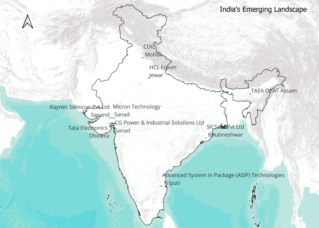
Geographically these plants are located in few selected cluster, for Example- In western India Sanad near Ahmedabad in Gujarat has 4 Plants, In south, Triputi in Andhara Pradesh has one facility under construction, In South-east, Bhubneshwar in Orissa has 2 Plants, In east Guwahati has one facility and north one facility is in Jewar Uttar Pradesh and one Chandigarh UT. Each of these facility is located in unique climatic zone differing strongly from one another.
In Semi Conductor production facility Temperature, Humidity, Water etc play critical role, in deciding location and cost per unit. Our climatic data analysis suggest that each of location has its own strength and weakness.
Temperature, Humidity and Water
- Temperature conditions show that Ahmedabad and Tirupati experience the highest thermal stress. both stations record mean daily maximum temperatures above 34 °C and extreme maximum temperatures exceeding 43 °C.
- Ahmedabad further stands out due to its large diurnal temperature rise, indicating strong daytime heat loading and high peak cooling demand. in contrast, Bhubaneswar records slightly lower mean maximum temperatures, while Guwahati remains the coolest site with a mean daily maximum of around 30 °C and substantially lower extreme temperatures.
- From an operational perspective, inland stations therefore face higher electricity demand and cooling infrastructure costs compared to coastal and northeast locations.
- Humidity patterns display an opposite gradient. Ahmedabad exhibits low daytime relative humidity and lower vapour pressure, suggesting limited moisture-related stress but high sensible cooling demand.
- Tirupati shows moderate humidity levels, implying a mixed cooling regime. Bhubaneswar and guwahati, however, maintain high relative humidity and vapour pressure throughout the day, indicating that cooling demand in these regions is dominated by latent heat removal and dehumidification rather than temperature reduction. this increases the importance of air handling and humidity control systems in coastal and northeast plants.
- Water availability introduces a third layer of contrast. ahmedabad receives the lowest annual rainfall and the fewest rainy days, making it structurally water-scarce and highly dependent on engineered water supply and recycling systems.
- Tirupati occupies an intermediate position with moderate rainfall and water reliability.
- Bhubaneswar and Guwahati receive high annual rainfall and a large number of rainy days, providing stronger natural water security. However, this abundance also brings challenges related to excess water, drainage, and weather-related disruptions, particularly in Guwahati where rainfall and storm activity are highest.
Thus taken together, the results indicate that no single location is climatically optimal for semiconductor manufacturing. dry inland locations face higher temperature and water costs, while humid and water-rich regions experience higher moisture-related cooling demand and operational disruption risks. the discussion highlights that site suitability for semiconductor plants in india depends on balancing temperature-driven energy costs, humidity-driven dehumidification requirements, and water-related infrastructure and reliability considerations.
Cost Implication of Temperature, Water and Climate
Temperature, Humidity and Cost
Based on the total cooling load index, cooling-related energy costs at Ahmedabad are about 64% higher than tirupati, 214% higher than Guwahati, and around 240% higher than Bhubaneswar. In other words, cooling at Ahmedabad is more than three times as energy intensive as at Bhubaneswar and Guwahati. Tirupati represents an intermediate-cost location, with cooling demand roughly 92% higher than Guwahati and about 110% higher than Bhubaneswar, but still significantly lower than Ahmedabad.
Bhubaneswar and Guwahati show the lowest total cooling load, yet their costs are not negligible, as a larger share of energy use is directed toward humidity control rather than temperature reduction. Thus, while dry inland locations incur sharply higher temperature-driven cooling costs, humid regions shift the cost burden toward latent cooling and dehumidification, highlighting distinct but equally important operational challenges.
Water and Cost
Ahmedabad shows the highest water stress, with a precipitation reliability (PR) of only 0.093, meaning rainfall occurs on less than 10% of days in a year. as a result, its water scarcity index (WSI) is 0.907, which is about 7% higher than Tirupati, 13% higher than Bhubaneswar, and 20% higher than Guwahati. the water infrastructure multiplier (WIM) for Ahmedabad is 1.907, indicating that water-related infrastructure and operational costs are nearly 91% higher than a fully water-secure location. its recycling pressure index (RPI) is the highest at 31.2, reflecting strong dependence on water recycling and engineered supply systems.
Tirupati represents an intermediate case. its precipitation reliability of 0.151 is about 62% higher than Ahmedabad, reducing water scarcity pressure, yet its WSI of 0.849 still implies substantial dependence on managed water infrastructure. compared to Guwahati, Tirupati’s water scarcity is about 13% higher, and its recycling pressure remains significant.
Bhubaneswar and Guwahati show much lower water cost pressure. Bhubaneswar’s precipitation reliability (0.20) is more than double that of Ahmedabad, reducing water scarcity by about 12% relative to Tirupati. Guwahati is the most water-secure site, with precipitation reliability of 0.247, nearly 2.7 times higher than Ahmedabad, and the lowest WSI (0.753). Consequently, Guwahati’s recycling pressure index is about 28% lower than Ahmedabad.
Overall, water-related costs at Ahmedabad are likely to be 20–30% higher than Tirupati and 40–45% higher than Bhubaneswar and Guwahati, driven by low rainfall reliability and high dependence on recycling and infrastructure. while eastern and northeastern locations benefit from natural water availability, their challenge lies less in scarcity and more in managing excess water and rainfall variability.
Operational Disruption Cost
Ahmedabad records a WDI of 24.9, reflecting relatively low fog incidence and moderate thunder activity. This suggests that weather-related operational disruptions are limited and largely manageable, with risks concentrated more on air quality and heat than on visibility or storm events.
Tirupati shows a slightly higher WDI of 28.4, about 14% higher than Ahmedabad. This increase is driven by more frequent fog days combined with similar thunder activity, indicating a modest rise in weather-related operational interruptions.
Bhubaneswar records a WDI of 29.5, roughly 18% higher than Ahmedabad. the higher value reflects increased fog occurrence and regular thunder activity, suggesting a greater likelihood of short-term disruptions to logistics and outdoor operations, particularly during the monsoon season.
Guwahati stands out sharply with a WDI of 99.2, which is nearly four times higher than Ahmedabad and more than three times higher than Tirupati and Bhubaneswar. this very high value is driven by frequent thunderstorms and persistent fog, indicating significant operational risk related to visibility loss, transport delays, and weather-induced downtime.
Limitation of Study
This study relies on climatological averages and selected station data, which may not capture short-term extremes or local micro-climatic variation at plant sites. the cost indices used are relative proxies and do not represent actual monetary costs due to the absence of plant-level energy, water, and tariff data. non-climatic factors such as infrastructure quality, technology efficiency, and policy support are not included, and future climate change impacts are not explicitly considered.